From Compression Test to Curve Fitting Analysis: Hyperelastic Rubber-Like Material
Fares Al Rwaihy
May 26, 2023
225
1
Exploration of a hyperelastic rubber-like material with the goal of utilizing our compression test data for meaningful application in Finite Element Analysis (FEA).
4 min read
Introduction
In this post, we will explore the journey from conducting a compression test to performing a curve fitting analysis on a hyperelastic rubber-like material. Through meticulous data collection and analysis, we were able to successfully complete our project, (Investigating Hyperelastic Behavior of 3D Printed Rubber-like Material).
Results of compression test
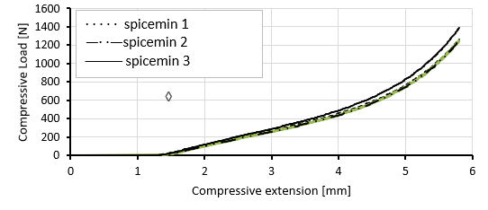
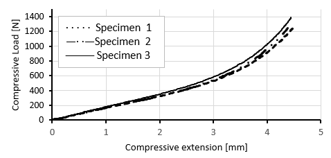
After conducting the compression test, we obtained experimental data in an Excel file that contained all the necessary values for our evaluation. The analysis involved three different specimens subjected to four different Compressive Load-Compressive Extensions loading and unloading paths, the results of the 3rd specimen shown in the figure.
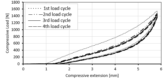
Upon examining the data, it became evident that the first cycle exhibited a distinct behavior due to the compressive load-compressive extension characteristics of the rubbery material. This behavior was unique and not repeated as the material softened.
The other three cycles were the same, thus we could shorten the analysis period by only considering the fourth cycle's loading path of each specimen.
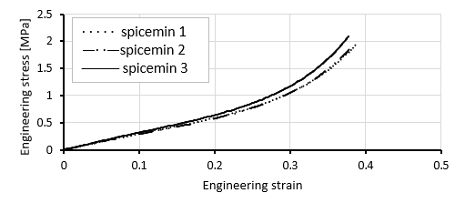
Plotting the stress-strain graphs
Stress-Strain graphs are the most necessary graphs needed for curve fitting thus additional work on Compressive Load-Compressive Extension graphs is required to shift the graphs to the origin. Assuming an ideal case where compression is homogeneous and there is no slip between the metal plates and the test specimens as well as the shape of the test specimens and all other circumstances considered to be ideal. Under slight deformation, there must be a linear relationship in the compressive load-compressive extension graphs.
However, results showed approximate zero values of compressive force until 1.3 mm where the linear relationship starts to occur. To overcome this challenge, we adopted the following approach:
- A trend line was selected to represent the general trend of the data.
- A linear equation was obtained to describe the trend line.
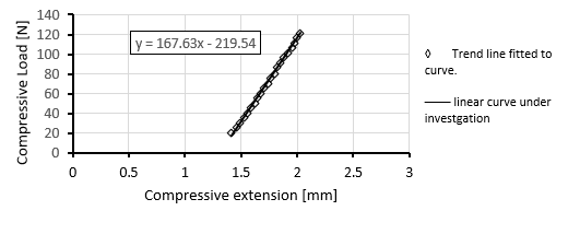
- To shift the curve to the origin, the X value was determined by subtracting the corresponding y value equal to zero.
- The experimental data values were then adjusted by subtracting the X value, effectively shifting the curve.
By implementing this technique, and using of the following equations
The engineering stress:
The engineering strain:
Stretch ratio:
We were able to plot the stress-strain curves accurately, ensuring that the data aligned with the appropriate reference point. This enabled us to further analyze and interpret the material's behavior with confidence.
Curve fitting
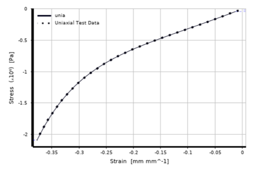
To accurately characterize our printed material, we conducted the curve fitting process using ANSYS Workbench software. The methodology for performing the curve fitting consisted of the following steps:
- Transferring the stress-strain data values obtained from the experimental data into the software.
- Selecting different types of hyperelastic material models available within the software.
- The curve fitting process yielded constants ( C ) that could be interpreted as material properties, which can be obtained by using one of these from many hyperelastic material models.
Yeoh:
Mooney-Rivlin:
Neo‐Hookean:
The results of the curve fitting process were highly promising, as one of the generated curve closely matched the experimental data curve. This alignment between the two curves indicated that the generated constants successfully captured the material's behavior, validating their suitability for further research and analysis.