Heat Transfer Analysis
Fares Al Rwaihy
May 16, 2023
93
0
This series of blog posts aims to compare the hand calculation and numerical simulation techniques through technical softwares
4 min read
Introduction:
Heat transfer is an important aspect of many engineering applications, ranging from electronic cooling to thermal management in buildings. Accurately predicting heat transfer rates and temperatures is crucial for optimizing system performance and ensuring reliability.
Objectives:
The main objective of this series of blog posts is to compare hand calculation and numerical simulation techniques in heat transfer. We will discuss the role of technical software, such as finite element analysis (FEA), in accurately simulating complex heat transfer phenomena. By the end of this blog, readers will have a deeper understanding of heat transfer and the techniques used to analyze and optimize heat transfer systems.
Overview
Heat transfer is the exchange of thermal energy between physicals systems. A physical system is a region of space bounded by a closed surface and filled with a physical substance (medium) which could be a solid, liquid, or gaseous.
However, the amount of heat transferred through a cross section are (A) at moment (t) is defined as following:
In case of Steady-State heat transfer the amount of heat intensity remains constant along the cross section are (A). Furthermore in order for the heat to be transferred, three modes of transforming which are Conduction, Convection, and Radiation.
**Conduction and Convection can be only released, if the transfer space is filled with a medium which is not necessary for radiation which could be transferred in a vacuum
Steady-State thermal conduction
Thermal conduction equation
Heat is transferred from a hotter region of the intervening medium to a colder one through collisions between neighboring objects such as molecules, atoms, or electrons.
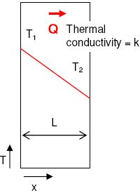
It follows this equation
where k is the thermal conductivity of the intervening medium, thus the thermal resistance R can be introduced
Thermal resistance in series vs parallel
in Series:
in Parallel:
Steady-State thermal convection
On the other hand, convection is not the transfer of heat within the layers of a material, but rather the transfer of heat between a surface and the surrounding medium through fluid flow.
It follows this equation
where α is the convection heat transform coefficient of the intervening medium, thus the thermal resistance R can be introduced
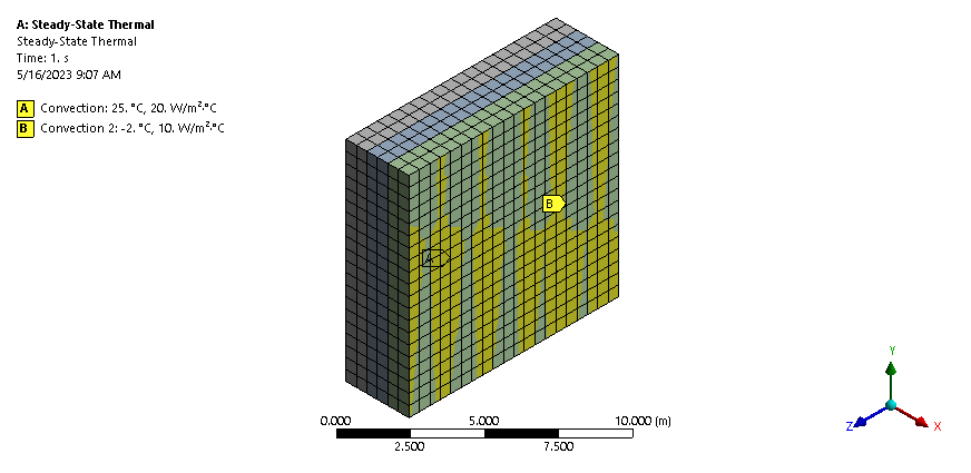
Steady-State thermal FEA simulation
Problem Setup
The simulation below shows the composite wall of a cold store. The outer layer of the wall is made of structural steel while the inner one is of Aluminum.
Results
As a result of the analysis, a chart is provided that indicates the variation of temperature with the distance along the wall layers.
Hand Calculation
Total thermal resistance
Heat intensity through the wall
Calculate T1, T2, T3 surface temperature
we will first calculate the temperature drop between the ambient air and the surface of the composite wall, from T0 to T1 then T1 to T2....etc
Using the same principle
Discussion
The agreement between the software simulation and hand calculation in predicting temperatures is a significant achievement. It validates the accuracy and reliability of both methods, highlighting the effectiveness of numerical techniques in modeling heat transfer. This convergence of results enhances our understanding of heat transfer mechanisms and supports the practical use of numerical simulations in engineering applications.